Kernel Density Estimation
Working with several animals/instances
- Adjusting animal specific parameters

Kernel Density Estimation

Most steps that are available from the GUI can also be called from the command line.

library(rhr)
data(datSH)
str(datSH)

## 'data.frame':    1500 obs. of  5 variables:
##  $ collar     : chr  "c5182" "c5182" "c5182" "c5182" ...
##  $ x_epsg31467: int  3558403 3558548 3558541 3558453 3558566 3557836 3557881 3557150 3557021 3555975 ...
##  $ y_epsg31467: int  5999400 5999099 5999019 5999026 5999365 5999185 5999139 5999159 5998865 5997615 ...
##  $ day        : chr  "2009-02-13" "2009-02-13" "2009-02-13" "2009-02-13" ...
##  $ time       : chr  "00:02:23" "06:02:21" "12:01:51" "18:00:55" ...

We see that x and y coordinates are saved in the second and third column. Next we will perform a KDE.

kd1 <- rhrKDE(datSH[, 2:3])

## rhrRasterFromExt: using equal nrow and ncol

The kde functions take three additional arguments: bandwidth, template raster and levels.

Bandwidth

The bandwidth can be provided as a vector of length one or two. Several methods to estimate bandwidth are available.

rhrHref: estimates the reference bandwidth.
rhrHlscv: estimates the least square cross validation bandwidth.
rhrHpi: estimates the plug in the equation bandwidth.
rhrHrefScaled: estimates a scaled re fence bandwidth (as described in @Kie2013)

The default bandwidth is the reference bandwidth.

## Calculating reference bandwidth:
(href <- rhrHref(datSH[, 2:3]))

## $h
## [1] 618.104 618.104
## 
## $rescale
## [1] "none"

## Or plugin the equation
(hpi <- rhrHpi(datSH[, 2:3]))

## $h
## [1] 65.04826 74.39719
## 
## $rescale
## [1] "none"
## 
## $correct
## [1] TRUE

kdehref1 <- rhrKDE(datSH[, 2:3], h = href$h)

## rhrRasterFromExt: using equal nrow and ncol

kdehref2 <- rhrKDE(datSH[, 2:3], h = rhrHref(datSH[, 2:3])$h)

## rhrRasterFromExt: using equal nrow and ncol

## Are they the same
identical(rhrUD(kdehref1), rhrUD(kdehref2))

## [1] TRUE

Working with the result

Once we successfully estimated a KDE, there are several things we can do with. The first thing might be to plot it:

plot(kdehref1)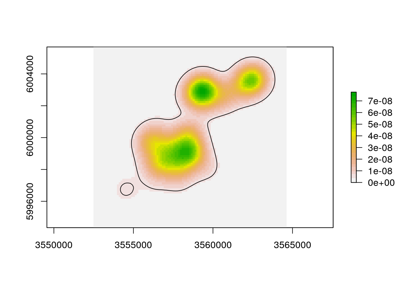

The functions rhrUD and rhrIsopleths allows to retrieve the UD and isopleths respectively.

ud <- rhrUD(kdehref1)
class(ud)

## [1] "RasterLayer"
## attr(,"package")
## [1] "raster"

The ud is a RasterLayer from the raster package. Similarly we can obtain the the isopleths at a predefined or specific level.

## the default level of 95
iso1 <- rhrIsopleths(kdehref1)
plot(iso1)

class(iso1)

## [1] "SpatialPolygonsDataFrame"
## attr(,"package")
## [1] "sp"

## other levels
iso2 <- rhrIsopleths(kdehref1, levels = seq(10, 90, 5))
plot(iso2)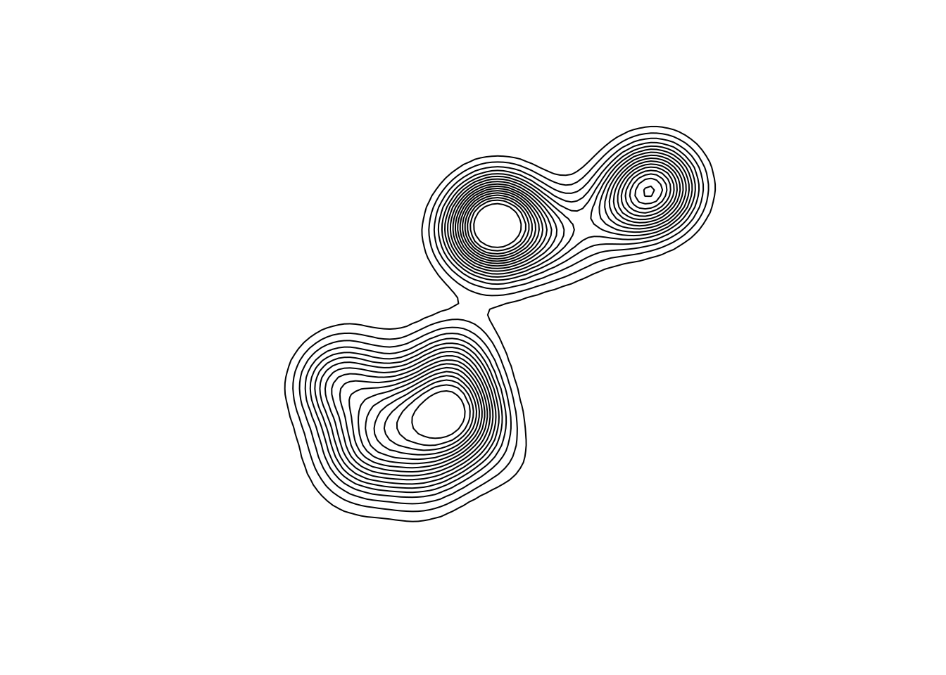

The rhrArea functions returns the home-range area at a given isopleth.

## default level
rhrArea(kdehref1)

##   level     area
## 1    95 38325055

## other levels
rhrArea(kdehref1, levels = seq(10, 90, 5))

##    level     area
## 1     10  1401063
## 2     15  2203714
## 3     20  3089250
## 4     25  4019084
## 5     30  5011304
## 6     35  6069462
## 7     40  7215234
## 8     45  8435629
## 9     50  9771290
## 10    55 11211624
## 11    60 12819124
## 12    65 14571133
## 13    70 16664247
## 14    75 18931113
## 15    80 21714672
## 16    85 25249938
## 17    90 30171443

Saving results

Isopleths can be saved various GIS formats, e.g.,

raster::shapefile(iso1, "myShape.shp")

Working with several animals/instances

Often it may be useful to work with more than one animal or instance (i.e., different tracking periods of the same animal) simultaneously. rhr does not provide direct support for this. However, it can be easily achieved using base R.

As an example, we will estimate monthly home ranges for the example red deer data set datSH. To do this we have to go through 3 steps:

Define a factor to split the data (e.g., species id, month of the year, study area).
Split the data with R’s split function.
Apply some home range estimate.

library(rhr)
library(lubridate)
data(datSH)

# 1. define a splitting variable, here I will use the months
datSH$month <- round_date(ymd(datSH$day), "month")

# 2. Split the data
dat2 <- split(datSH, datSH$month)

# 3. Apply home range estimates
hrs <- lapply(dat2, function(x) rhrKDE(x[, 2:3]))  # x is now the data for 1 month

## rhrRasterFromExt: using equal nrow and ncol
## rhrRasterFromExt: using equal nrow and ncol
## rhrRasterFromExt: using equal nrow and ncol
## rhrRasterFromExt: using equal nrow and ncol
## rhrRasterFromExt: using equal nrow and ncol
## rhrRasterFromExt: using equal nrow and ncol
## rhrRasterFromExt: using equal nrow and ncol
## rhrRasterFromExt: using equal nrow and ncol
## rhrRasterFromExt: using equal nrow and ncol
## rhrRasterFromExt: using equal nrow and ncol

hrs is now a list where each entry is the kernel density estimate for one month. To obtain the home range size (HRS) of the first month, we can use:

rhrArea(hrs[[1]])

##   level   area
## 1    95 774638

and with sapply we can easily obtain the home range size for all months.

sapply(hrs, rhrArea)

##       2008-04-01 2008-05-01 2008-06-01 2008-07-01 2008-08-01 2009-01-01
## level 95         95         95         95         95         95        
## area  774638     9727988    21492189   5226063    3799606    502955.9  
##       2009-02-01 2009-03-01 2009-04-01 2009-05-01
## level 95         95         95         95        
## area  7797540    15470853   7508145    7501840

Adjusting animal specific parameters

If, e.g., parameters such as the bandwidth should be instance specific there are two ways:

Estimate the parameters for each instance.
Estimate the parameter on the fly.

Adjusting the example from above we get:

library(rhr)
library(lubridate)
data(datSH)

dat2 <- split(datSH, round_date(ymd(datSH$day), "month"))
bw <- lapply(dat2, function(x) rhrHpi(x[, 2:3]))
hrs <- lapply(seq_along(bw), function(i) rhrKDE(dat2[[i]][, 2:3], h = bw[[i]]$h))

## rhrRasterFromExt: using equal nrow and ncol
## rhrRasterFromExt: using equal nrow and ncol
## rhrRasterFromExt: using equal nrow and ncol
## rhrRasterFromExt: using equal nrow and ncol
## rhrRasterFromExt: using equal nrow and ncol
## rhrRasterFromExt: using equal nrow and ncol
## rhrRasterFromExt: using equal nrow and ncol
## rhrRasterFromExt: using equal nrow and ncol
## rhrRasterFromExt: using equal nrow and ncol
## rhrRasterFromExt: using equal nrow and ncol

We could also do this on the fly with

dat2 <- split(datSH, round_date(ymd(datSH$day), "month"))
hrs <- lapply(dat2, function(x) rhrKDE(x[, 2:3], h = rhrHpi(x[, 2:3])$h))

## rhrRasterFromExt: using equal nrow and ncol
## rhrRasterFromExt: using equal nrow and ncol
## rhrRasterFromExt: using equal nrow and ncol
## rhrRasterFromExt: using equal nrow and ncol
## rhrRasterFromExt: using equal nrow and ncol
## rhrRasterFromExt: using equal nrow and ncol
## rhrRasterFromExt: using equal nrow and ncol
## rhrRasterFromExt: using equal nrow and ncol
## rhrRasterFromExt: using equal nrow and ncol
## rhrRasterFromExt: using equal nrow and ncol

Using the command line