File upload size exceeded

shiny limits file uploads by default to 5MB per file. This can be changed with the following command:

options(shiny.maxRequestSize=30*1024^2)

Now it would be possible to upload files up to 30MB (see here for more)

Why is buffer width important?

The question how to chose the right output grid buffer and resolution and if the choice matters has come up several time. We try to illustrate some of the points with a simulated set of relocations and kernel density estimation (KDE).

First we simulate a series of relocation with a random walk.

library(rhr)

set.seed(1984)
n <- 1000

## simulate dummy data
path <- data.frame(x = cumsum(rnorm(n)), y = cumsum(rnorm(n)))
plot(path, type = "l", asp = 1)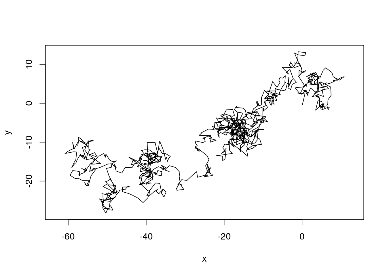

Next we will create four different template grids with two different buffer widths and resolutions.

b <- list(
  rhrRasterFromExt(rhrExtFromPoints(path, buff = 10), res = 1), 
  rhrRasterFromExt(rhrExtFromPoints(path, buff = 200), res = 1), 
  rhrRasterFromExt(rhrExtFromPoints(path, buff = 10), res = 10), 
  rhrRasterFromExt(rhrExtFromPoints(path, buff = 200), res = 10)
)

bbx <- lapply(b, function(x) rgeos::gEnvelope(SpatialPoints(t(bbox(x)))))

plot(bbx[[4]], border = "black", main = "Buffers")
plot(bbx[[3]], border = "red", add = TRUE)
points(path)
axis(1)
axis(2)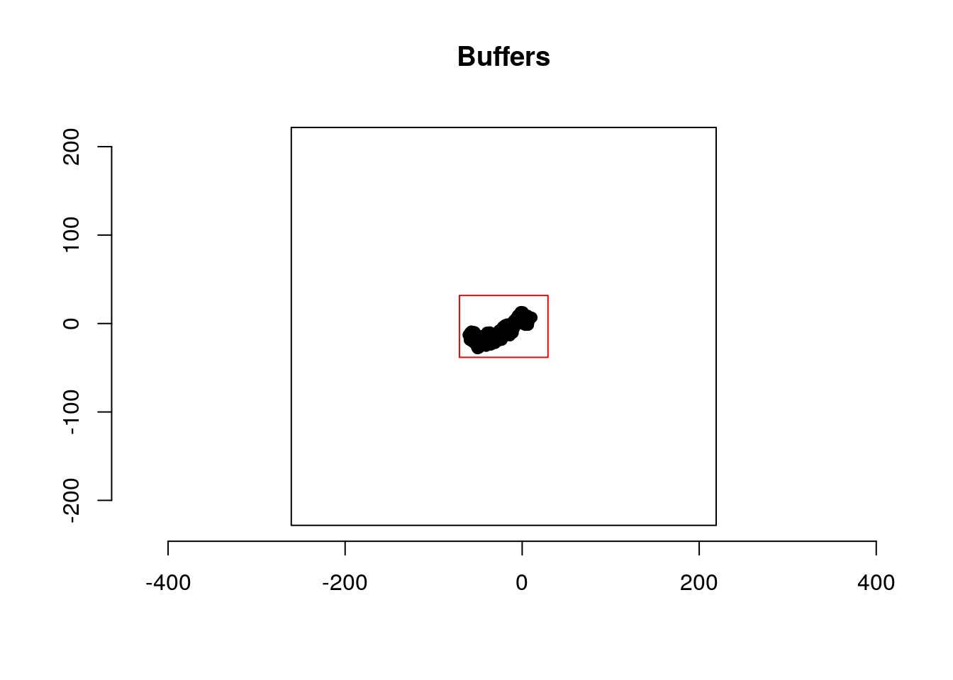

Next we can estimate KDE and plot them.

kdes <- lapply(b, function(x) rhrKDE(path, trast = x))
par(mfrow = c(2, 2))
lapply(kdes, function(x) plot(rhrUD(x), legend = FALSE))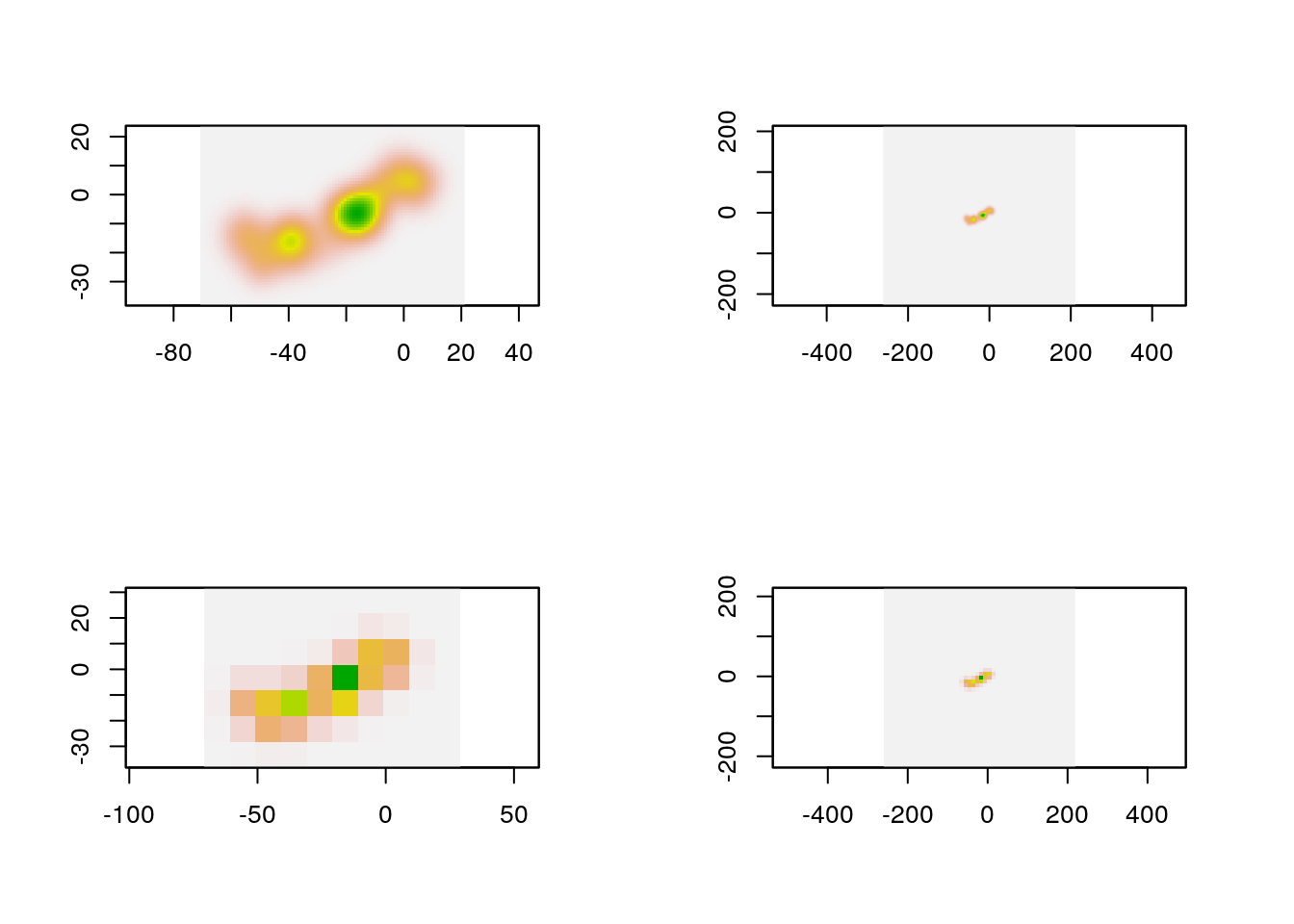

Lets have a look at the home-range area:

sapply(kdes, rhrArea)

##       [,1]    [,2]    [,3]     [,4]    
## level 95      95      95       95      
## area  1839.55 1899.88 1968.614 2385.633

We would expect all for areas to be equal, but they are not. We see that differences are smaller between the first two elements than the last two elements. If we plot the isopleths that are used to compute the areas it becomes clearer why this maybe the case.

par(mfrow = c(2, 2))
sapply(kdes, plot, legend = FALSE)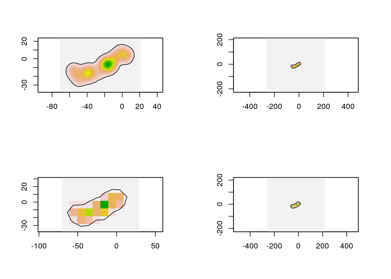

Plotting the isopleths from the different scenarios in one plot makes it even clearer.

par(mfrow = c(1, 1))
plot(rhrIsopleths(kdes[[4]]), lty = 2, border = "red")
plot(rhrIsopleths(kdes[[1]]), add = TRUE)
plot(rhrIsopleths(kdes[[2]]), lty = 2, add = TRUE)
plot(rhrIsopleths(kdes[[3]]), lty = 1, border = "red", add = TRUE)
legend("topleft", lty = c(1, 2, 1, 2), col = c("black", "black", "red", "red"), 
       legend=c("Buffer = 10; Resolution = 1", "Buffer = 200; Resolution = 1", 
                "Buffer = 10; Resolution = 10", "Buffer = 200; Resolution = 10"))
axis(1)
axis(2)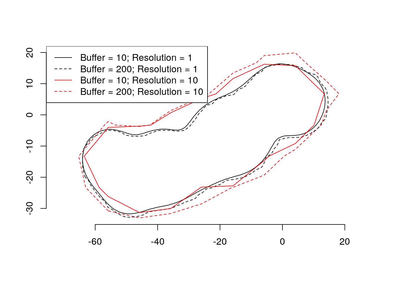

What does this mean?

• Larger buffers tend to produce larger estimates of home-range areas.
• The effect of buffer width is stronger with lower resolution (i.e., larger pixels).
• Estimates of home-range area are less sensitive to buffer width than to resolution.

Effect of buffer and resolution on bandwidth

Consider the following example

library(rhr)
data(datSH)

h1 <- rhrHrefScaled(datSH[, 2:3]) # the default

## rhrRasterFromExt: using equal nrow and ncol

h2 <- rhrHrefScaled(datSH[, 2:3], trast = rhrRasterFromExt(rhrExtFromPoints(datSH[, 2:3], extendRange = 0.8), nrow =
  100, res = NULL)) # the default

## rhrRasterFromExt: using equal nrow and ncol

h1

## $h
## [1] 707.8309
## 
## $success
## [1] TRUE
## 
## $niter
## [1] 13

h2

## $h
## [1] 681.1043
## 
## $success
## [1] TRUE
## 
## $niter
## [1] 13

This also impacts the area of a KDE estimate:

rhrArea(rhrKDE(datSH[, 2:3], h = h1$h))

## rhrRasterFromExt: using equal nrow and ncol

## Warning in rhrKDE(datSH[, 2:3], h = h1$h): rhrKDE: same bandwidth is used
## in x and y direction

##   level     area
## 1    95 43013574

rhrArea(rhrKDE(datSH[, 2:3], h = h2$h))

## rhrRasterFromExt: using equal nrow and ncol

## Warning in rhrKDE(datSH[, 2:3], h = h2$h): rhrKDE: same bandwidth is used
## in x and y direction

##   level     area
## 1    95 41660242

We can change the results further by changing the extent of the raster

rhrArea(rhrKDE(datSH[, 2:3], trast = rhrRasterFromExt(rhrExtFromPoints(datSH[, 2:3], extendRange = 0.8), nrow =
  100, res = NULL), h = h1$h))

## rhrRasterFromExt: using equal nrow and ncol

##   level     area
## 1    95 43450498

rhrArea(rhrKDE(datSH[, 2:3], trast = rhrRasterFromExt(rhrExtFromPoints(datSH[, 2:3], extendRange = 0.8), nrow =
  100, res = NULL), h = h2$h))

## rhrRasterFromExt: using equal nrow and ncol

##   level     area
## 1    95 41959392